How to Highlight a Row in Google Sheets Based on a Checkbox

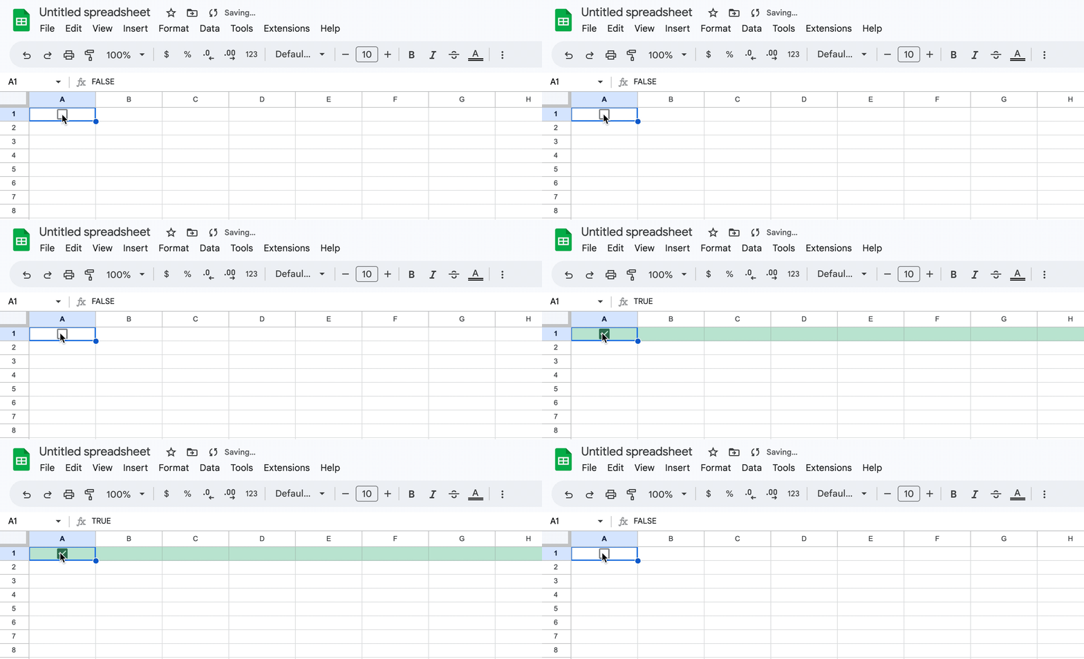
Have you ever considered using Google Sheets to perform the following action: clicking on a checkbox causes the entire row to become highlighted in a color of your choice? This can be extremely useful for marking specific tasks as completed.

Here is a step-by-step guide on how to achieve this.

Step 1

First, make sure you have checkboxes in your sheet. If not, you can add them by clicking the cell where you want a checkbox, then going to “Insert” in the top menu and selecting “Checkbox.”

Step 2

Once you have your checkboxes set up, you can create a new conditional formatting rule. To do this, click on “Format” in the top menu, then select “Conditional formatting.“

Step 3

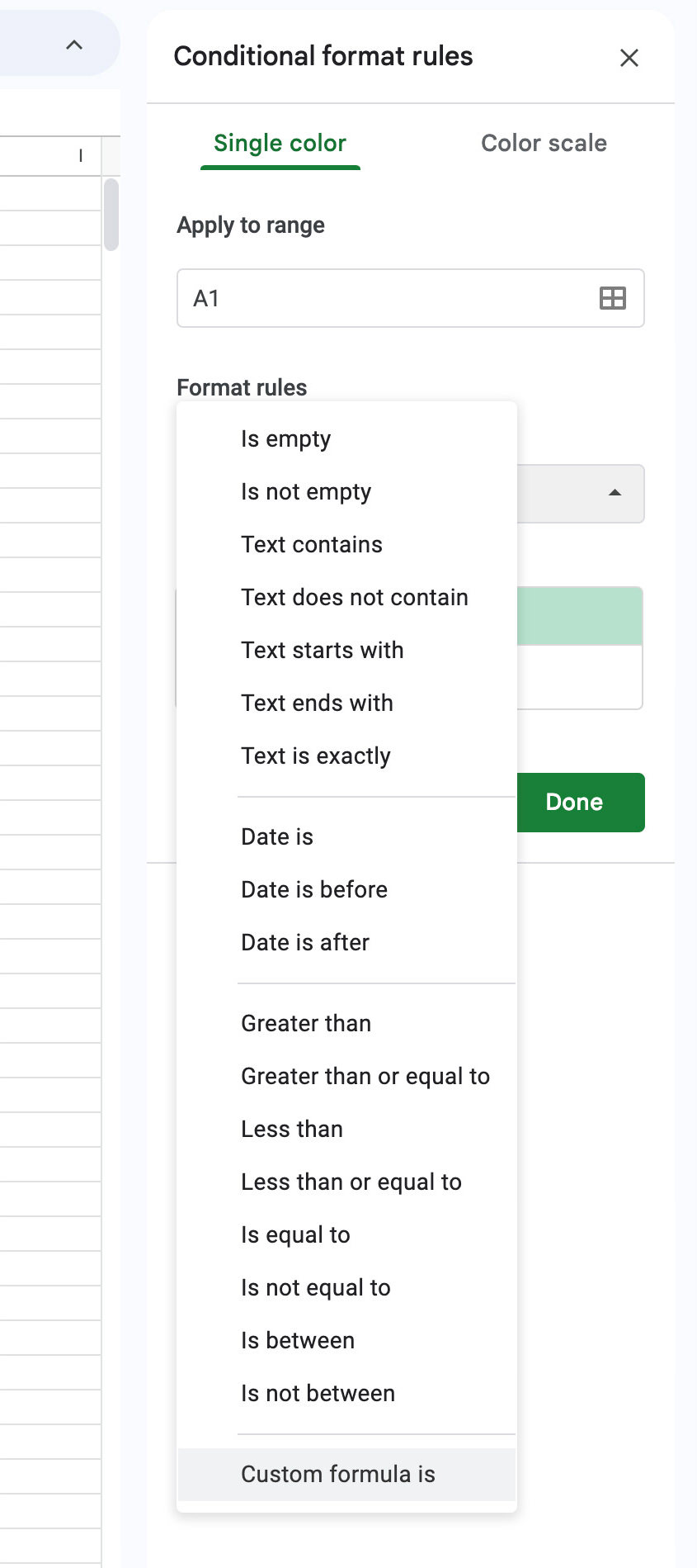
In the conditional formatting panel that opens on the right side, under the “Format cells if” drop-down, select “Custom formula is.“

Step 4

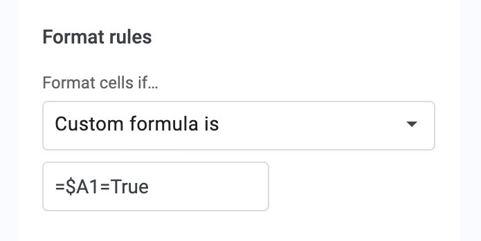
In the field below, enter a formula that references the cell with the checkbox. If your checkbox is in column A and you want to apply this to the whole sheet, you would write =$A1=True. The dollar sign ($) before A makes the column absolute, so it won’t shift when applied to the whole row, and 1 should be the first row number of your data range.

Step 5

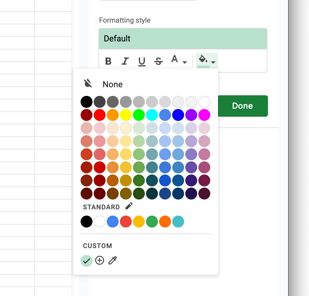
After entering the formula, select the formatting style you want to apply when the checkbox is checked. You can set the background color, text color, and more. In this case, we will change the background color to green, as an accomplished task is usually associated with the green color.

Step 6

Finally, under “Apply to range“, enter the range where you want this rule to apply.

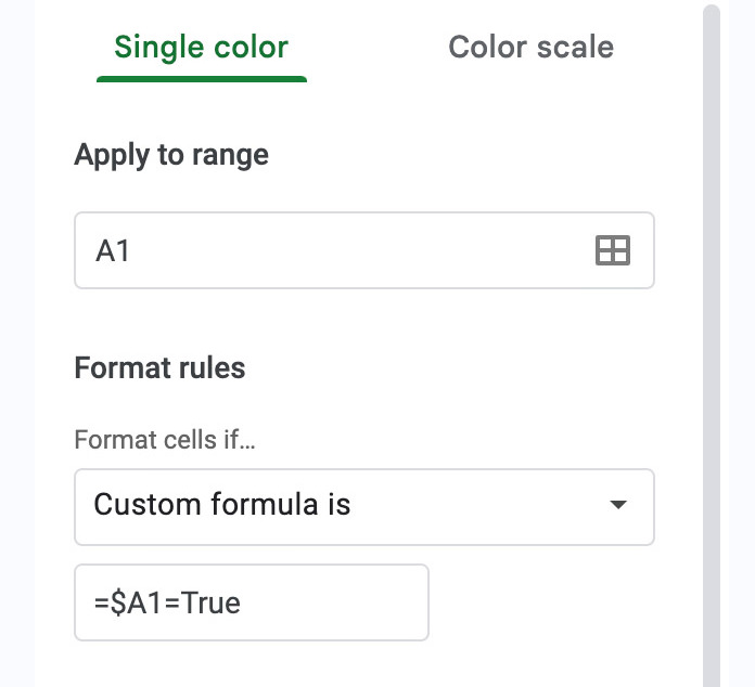
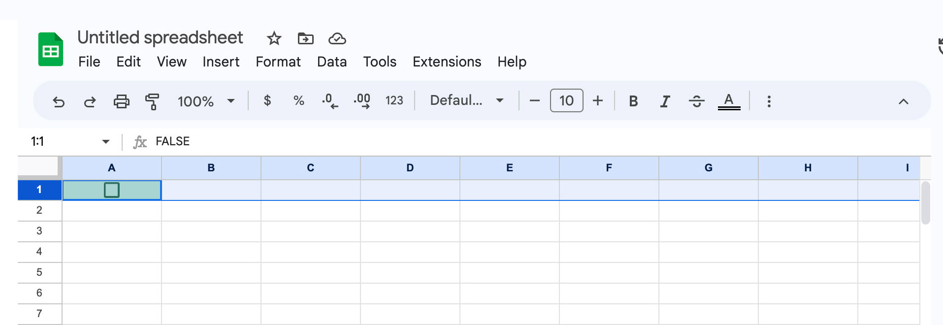
If you want it to apply to the entire row, just click on the row number on the left and the entire row will be selected.

Step 7

Click “Done” to apply the rule. Here’s what it looks like when you click on the checkbox.